Transformation of the Transformer

draft

February 10, 2026 · 6 min read

"Attention is all you need" might be the most influential paper in the past decade. The transformer has completely transformed (you can't stop me) AI and is now everywhere.

Naturally, it has also undergone several updates and improvements since its release. And this post is meant to track that.

Timeline: Papers and Models

TBD

Placeholder

TODO: add details.

When I first looked up mixture of expert models, I was quite confused. Switch transformers had already been around for a really long time!

We are going to organize all the research (and their adoption into open source models) all in one place so we can how things have evolved (...)

...

This is not a beginner's guide, but some useful refreshers and beginner friendly content is inserted in between.

The Base Transformer

Attention is All You Need introduced two key things:

Scaled Dot Product Attention (which is one of many types of attention, btw)
Mutli-Head Attention (MHA)

Both of these are components in the "base implementation" of the vanilla transformer. We will therefore use these to establish our context and terms.

Scaled Dot Product Attention

This attention mechanism uses a triplet of matrices: the query matrix $Q$ , the key matrix $Q$ , and the value matrix $V$ . Each matrix computed by embedding the input token sequence $X$ . The output of this attention mechanism is a weighted sum of the value vectors $v_i$ , where the weights are the dot product between the query and key pairings:

\text{Attn}(\mathbf{Q}, K, V) = \text{SoftMax}(\frac{QK^{\mathsf{T}}}{\sqrt{d_k}})V

In other words, for each pair of $q_i$ and $v_j$ , we get the following "score":

a_{i,j} = \text{SoftMax}(\frac{q_i k_j ^{\mathsf{T}}} {\sqrt{d_k}})

And so for the $i$ th input token, we get a vector representing scores of all tokens pairs (that came before*) and can compute a linear combination of all value embeddings for the $i$ ith token.

[a_{i,1} ... a_{i,L}] V = [a_{i,1} ... a_{i,L}] [v_{1} ... v_{L}]^{\mathsf{T}}

Put another way, this linear combination describes how all the other embeddings are allowed to "infleunce" our token's embedding. Low scores = low influence, high scores = high influence.

It's a dynamic weighing based on the input tokens!

*Notice also that we usually adopt causal attention. i.e. tokens can only be attended to by tokens from before rather than after (no peeking!)

Let's now establish our vocabulary of terms:

Symbol	Meaning
$d$	Model size / hidden dimension.
$\mathbf{X} \in \mathbb{R}^{L \times d}$	Input sequence embeddings.
$\mathbf{W}^q \in \mathbb{R}^{d \times d_k}$	Query projection matrix.
$\mathbf{W}^k \in \mathbb{R}^{d \times d_k}$	Key projection matrix.
$\mathbf{W}^v \in \mathbb{R}^{d \times d_v}$	Value projection matrix.
$\mathbf{W}^o \in \mathbb{R}^{d_v \times d}$	Output projection matrix.
$\mathbf{W}_i^q, \mathbf{W}_i^k, \mathbf{W}_i^v$	Per-head projections (each with width $d_k/h$ or $d_v/h$ ).
$\mathbf{Q} = \mathbf{X}\mathbf{W}^q \in \mathbb{R}^{L \times d_k}$	Query matrix.
$\mathbf{K} = \mathbf{X}\mathbf{W}^k \in \mathbb{R}^{L \times d_k}$	Key matrix.
$\mathbf{V} = \mathbf{X}\mathbf{W}^v \in \mathbb{R}^{L \times d_v}$	Value matrix.
$\mathbf{q}_i, \mathbf{k}_i, \mathbf{v}_i$	Row vectors of $\mathbf{Q}$ , $\mathbf{K}$ , $\mathbf{V}$ .
$d_k, d_v$	Key/value projection dimensions.
$\mathbf{A} = \mathrm{softmax}(\mathbf{Q}\mathbf{K}^{\top} / \sqrt{d_k})$	Attention weight matrix.
$\mathrm{Attn}(Q, K, V)$	Scaled dot product attention output.
$a_{ij}$	Attention weight from query $i$ to key $j$ .
$\mathbf{P} \in \mathbb{R}^{L \times d}$	Positional encoding matrix.
$\mathbf{p}_i$	Positional encoding for token $i$ .
$\mathbf{x}_i$	Input embedding for token $i$ .

In PyTorch, this mechanism can be written like this:

def scaled_dot_product_attention(query, key, value):
  # we assume self-attention, and therefore the same source/target lengths
  sequence_length = query.size(-2)

  # for causal attention, we need a diagonal matrix as a mask
  mask = torch.ones(sequence_length, sequence_length).tril(diagonal=0)

  bias = (torch
          .zeros(sequence_length, sequence_length)
          .masked_fill(mask.logical_not(), float("-inf"))
          )

  scale_factor = 1 / math.sqrt(query.size(-1))
  weight = query @ key.transpose(-2, -1) * scale_factor # Q K^T / sqrt(dk)

  return torch.softmax(weight + bias, dim=-1) @ value

If you need a refresher or visualisation this section, I strongly recommend this 3blue1brown video:

Multi-Head Attention

To construct a model with dimension $d_{model}$ , we use multiple scaled dot product attention blocks in parallel, each receiving a chunk of the input with a dimension $d_{head}$ . This is such that $d_{model} = \text{num heads} \times d_{head}$

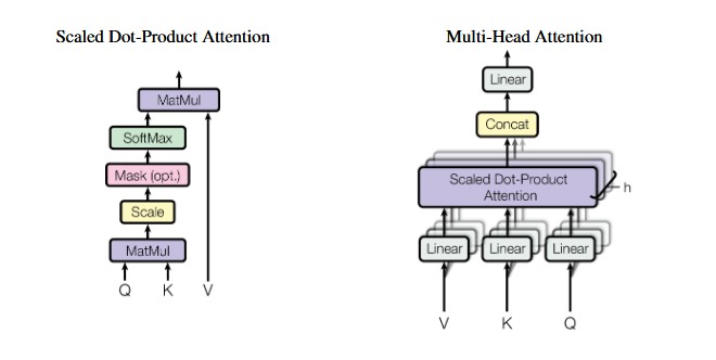
Figure — Transformer model architecture from 'Attention Is All You Need'.

With that, we have the building blocks of the original transformer model.

In this base state, we find that there are a few issues:

Each of $Q$ , $K$ and $V$ require matrix multiplications. Computing attention from these involves another 3 more matrix multiplies (not forgetting the final linear layer). It's expensive to compute.
Our current attention mechanism is positionally/permutationally invariant. That is, the positions of each token do not matter at all. We simply take a linear combination!

And we can also make it better too!

Hence begins the journey through the years of applying updates to the transformer

KV Caching and Paged Attention

The first big optimization to the attention block comes from the observation that we can "memo-ize" it. For every new input token we add to our sequence, we reuse practically all of the previous $K_{n-1}$ and $V_{n-1}$ matrices, needing only to add one additional vector.

We therefore cache all cache all "key" and "value" embeddings for all previous tokens during a generation.

But there's a little problem with this...

Memory Management for LLMs inference

Naively, if we were to store each of these key and value embeddings for a generation that can potentially reach $n$ tokens in sequence length, then we would have to allocate $2n$ tokens worth of contiguous memory. This is similar to pre-declaring and allocating memory to the maximum size of our arrays. And most of this could be potentially empty space! Perhaps the user just said "Hello" or "How many Rs are there in strawberry?". That's $2 * 100k$ tokens worth of space for each of these.

This is a large waste of memory during inference where we really can't anticipate memory requirements.

Enter paged attention. Instead of a contiguous block of memory for the KV cache, we chunk them into blocks. And then track each block using a block table. This block table is a mapping between token id series and memory addresses.

This means a few things:

Blocks need not be contiguous. We piece them together when needed. And only allocate memory when needed.
We can share blocks between queries. This is especially useful for constantly reused system prompts and other patterns of tokens. Blocks are a look up of token ids!

All of this translates to memory savings!

Grouped Query Attention

In Fast Transformer Decoding: One Write-Head is All You Need we take our memory savings further.

Instead of storing $N$ heads worth of KV caches, we group the heads into $G$ groups and have each group share a set of KV tensors. Hence, we slash memory by a factor of $N \divide G$ , i.e. the number of heads assigned to a group.

Multi-Head Latent Attention

Breaking away from the chronological progression... Multi-Head Latent Attention is a natural progression (and huge upgrade) from Grouped Query Attention.

Rotary Postion Embeddings (RoPE)

To deal with the issue of our attention mechanism being positionally invariant, we introduce the idea of positional embeddings into our transformer.